The CompSci's Guide To NOT Finding Bugs
This guide is not like the other guides in the series. There will be no bullet points on how to do things right, but instead I'll try to convince you that some things can never be done right. To be specific, I'll try to convince you to never use 'found bugs' as a form of scientific evidence.
TLDR: If you don't have time to read the full post, then the take away is that 'finding bugs' does not meet the requirements to qualify as scientific evidence and has some ethical problems in addition to that.
The rest of this post is concerned with an imaginary bug detection system ("DummyFuzz") which is being evaluated by "finding bugs". It doesn't matter what exactly DummyFuzz is doing, but let's just say we made some change to an existing fuzzer ("BaseFuzz"), and we want to study this effect. Also, DummyFuzz just happens to be based on random testing/fuzzing, but most of the arguments below also apply to static analysis or similar approaches.
The arguments below are presented in the following format. First, I'll present an evaluation description and conclusion as if it was written in a paper. I then point out the reasoning errors, and I then repeatedly try to fix them. The point of this exercise is to show that it is impossible to converge on a sound scientific experiment.
The main concerns I try to address are the basic requirements for a scientific experiment. The first is whether we can repeat and reproduce the experiment, which is the only way for other people to verify the data that backs up our claims. The next is falsifiability, that is whether the experiment can actually confirm or reject our theory depending on whether it is true. This is a fundamental idea behind science as running experiments to test our theory is the reason why scientists perform them.
Repeatability
Let's start with the simplest possible evaluation:
The first question is whether you could repeat or reproduce this? If you had access to DummyFuzz, you wouldn't know which software projects (or versions) to run it on, nor which bugs are expected to be found. You also don't know how long you even need to run it. The time description only mentions that the experiment run for a few months of real time, but the number of CPU hours is unclear.
Let's try to fix those simple errors first, which brings us to this evaluation:
Note: The changed text parts in each evaluation section are highlighted.
There are still two open issues that would prevent us from fully repeating this experiment. First, CPU hours are unfortunately not a good unit of measurement. One CPU hour contains more computations these days than 10 years ago, but there is not too much we can do to fix this in the current experimental setup.
Second, we would still need to find a way to map the found PoC from our fuzzer to the specific found bugs. This deduplication is usually done with some heuristics and or manually by the researchers or the developers of the target software. While the heuristics can be repeated, this manual root-cause analysis poses some difficulties, but let's just mark this down as a minor issue.
In the case of random testing, there is now the bigger question whether repeating this experiment will actually yield the same number of detected bugs. Given that random testing is based on randomness (duh), repeating experiments in the same environment might yield different results. The same setup might yield 0 bugs, 9 bugs, or any other higher number really if we base it all on just one trial.
To account for this, scientific reporting standards require you to account for noise via statistical tests and confidence intervals. For this we need to run several independent trials and then process the gathered data. Let's account for this in the next iteration of the evaluation:
At this stage the experiment is at least repeatable. We can't guarantee we see the same results in the paper due to the randomness, but we have an idea that in 95% of our experiments we should find a mean within the given confidence interval.
Falsifiability
The bigger question is now whether this experiment is reproducible? In other words, can you use the same approach to test the theory for yourself. To answer this, we also need to discuss when exactly this experiment confirms or rejects a tested theory (Falsifiability)?
Here the two fatal flaws of finding bugs in the wild come into play. The first flaw is that the whole experiment runs in an uncontrolled environment, which means that there is no guaranteed relationship between the found bugs and the veracity of the tested method.
To better illustrate this issue, assume that DummyFuzz is actually good at finding bugs and the evaluation should confirm the tested theory (i.e., we should find some bugs). Let's now say we can travel back in time, and we go back to the moment just before the evaluation above was started. We now manually search and fix all 9 bugs, and the evaluation will now reject DummyFuzz's theory as no bugs are found. In this scenario, we did not change anything about DummyFuzz at all, but just influenced the environment.
As an even more absurd situation, imagine that another researcher independently came up with the equivalent of DummyFuzz and runs their own evaluation just shortly before. They will now find 9 bugs, "confirm" their theory, while the following evaluation on the same target software cannot find any bugs and "rejects" the same theory.
One could argue that this issue could be partially solved by simply ignoring results on targets with no discoverable bugs. However, the problem with this solution is that we simply do not know which targets have no bugs. In fact, I do not recall any paper that ever disclosed the number of bugs that were not found using this approach, and I would not know how they could get this data.
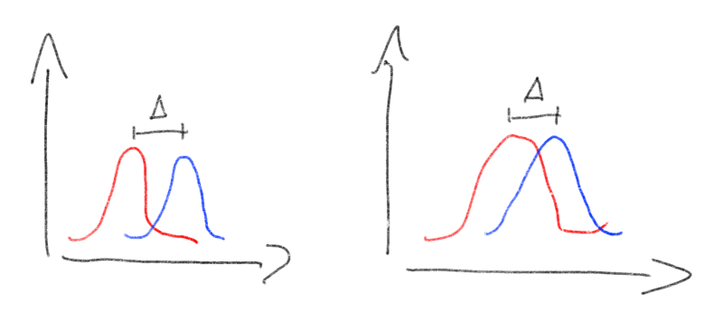
This is the second fatal flaw of finding bugs for the purpose of using it as scientific evidence: There are no negative outcomes provided that put the positive outcomes into context. If we look at the evaluation above, we could have found 9 bugs out of 9 existing bugs, which would be objectively a very good outcome. However, the same results are also obtained if we found 9 out of 1 million bugs, which most people would consider a rather bad result. In other words, it does not matter how many bugs you find, they are not evidence for any form of efficacy without negative cases.
State-of-the-art
One potential argument you might hear is that bug finding is still somewhat useful for showing some unknown relative progress towards the state of the art. Let's adjust the evaluation accordingly to get an example:
While this might sound reasonable at first, this line of reasoning unfortunately relies on two large assumptions. The first assumption is that all state-of-the-art bug detection tools are continuously used on the latest version of the target software and all bugs are reported. There is obviously no evidence that this is actually done, and given how many academic projects suffer from bit-rot and cannot be run at all, there is more evidence against this than in favor.
Additionally, this assumes that all bugs that are reported are fixed in an expeditious manner. This is obviously not true for most projects and you can easily see this for yourself by simply looking at the open issues in oss-fuzz.
What is especially worrying in this case is that this situation is very prone to incorrectly confirming wrong theories. Especially if the baseline is not given equal opportunity to find bugs, then this evaluation would also include the bugs detectable by the baseline. Given that the baseline was most likely used because it is already working well, and that most software includes at least some bugs, this approach can incorrectly confirm any change as beneficial.
Baselines
To fix the issue above, you might be inclined to narrow down the claim to only argue for an improvement over the baseline. Given that we most likely have a running baseline, we could even check for ourselves in the evaluation and no longer rely on vague assumptions. Let's fix this in the evaluation by also running the baseline and ending up with the following text.
Does this experiment now finally back up the conclusions we like to draw? The answer is still "no" as we cannot exclude the case that we merely shifted the detection capabilities of the baseline.
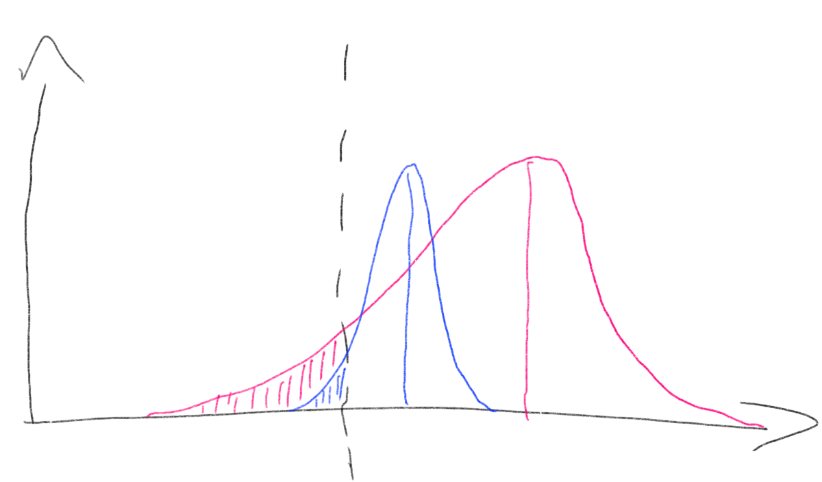
To give an example, let's assume that BaseFuzz can reliably find 90 of the unknown amount of bugs in the target, while DummyFuzz can find 19 bugs of which 10 are also detectable by its baseline BaseFuzz. Any reasonable experiment should identify that DummyFuzz is (a) worse than BaseFuzz and (b) only shifting detection capabilities around.
However, as said above, we are in an uncontrolled environment, so someone else might have already reported and fixed the 90 bugs by using the existing BaseFuzz. If that is the case, then in our evaluation would look like the text above where we claim that DummyFuzz can find 9 bugs while BaseFuzz finds 0. This inverts the actual truth that if given the choice between BaseFuzz and DummyFuzz, the baseline is substantially more useful.
In reality, the extreme case from above would not always happen as not all bugs are reported and fixed. But assuming a well-working and popular baseline (which is the ideal baseline for a prototype), we could get quite close to the scenario above.
Bug Finding as Non-Evidence
So far I mostly just pointed out basic scientific issues with this method, and there are plenty of more to write about (e.g., how representative are the found bugs or how we deal with optional stopping bias). However, I do want to address the argument that while bug finding is bad evidence, the process of gathering itself is beneficial. In other words, the found bugs itself provide a benefit to society and thus the method is not as flawed as it might look.
The argument against this is that there is no reason to conflate pro bono bug finding work with evidence in a paper. This same work could be done without presenting it as valid scientific evidence.
Arguably, this idea also misses the point of science which is about finding good solutions that can be adopted on a large scale by the public. In fact, the trade-off we are considering here seems very unbalanced. We trade the few bugs found by a few researchers for potentially misidentifying a non-working solution as better, which then causes the public to adopt it on a large scale (and miss many more bugs).
Ethical Issues
It does seem fitting to end this with a note about the thing that is most often forgotten in computer science: Ethics.
While ethics are often subjective, I think there are a some fundamental problem here that should be discussed. The biggest issue is arguably that reporting bugs is essentially outsourcing the evaluation work of papers towards the public. If you look at most papers, you can see that authors report all issues they find to open source projects. The developers of those projects are then doing all the work of deduplicating and triaging the respective issues.
It should be said that those developers are usually not credited on the respective papers for their work, nor is there any protocol in place for asking them for whether they consent to doing this work. In fact, I do not even see evidence that all developers are even aware they are doing this work for researchers. Many of the bug reports filed look like they are submitted by users who encountered a bug, or security researchers who are pentesting an application.
There is also a conflict of interest on the side of the researchers. If your paper evaluation gets more positive the more 'new' bugs you found, then the most successful course of action is to report as much as you can to the developers. When they fail to deduplicate a bug to a previously reported one, then that would make the evaluation more positive. In fact, the less information you provide the more likely it that they fail to find the correct previously reported bug.
In the same way, by not disclosing that the bugs are found
by an automated system and are not affecting an end user (and they
often do not affect end users
Conclusions
There isn't really more to say about this topic aside that this method is fundamentally flawed. Modern scientific fields such as medicine have long abandoned similar evaluation methods a long time ago, and computer science should have done the same decades ago. Why we haven't done this yet isn't the point of this post, but I hope that it convinced you at least of two things. First, you shouldn't use it in your paper. Second, you should not rely on it as evidence when judging the results of an existing paper.
References
[1] Marcozzi, Michaël, et al. "Compiler fuzzing: How much does it matter?." Proceedings of the ACM on Programming Languages 3.OOPSLA (2019): 1-29.
[2] Schloegel, Moritz, et al. "Confusing Value with Enumeration: Studying the Use of {CVEs} in Academia." 34th USENIX Security Symposium (USENIX Security 25). 2025.